A Phenomenological Background-Excitation Model of Light Propagation: The Impact-Triggered Flash Cascade (ITFC)

Full Text

The Impact-Triggered Flash Cascade (ITFC) Model: A Quantum-Interpreted Background Framework for Light Propagation

> Human Prompter

Koh, Hyun-Kyu

AI Co-Author

OpenAI GPT-5.4 Thinking

Version

GPT-5.4 Thinking

Role

Conceptual elaboration, structural drafting, editorial refinement, and formulation assistance

under the interactive persona “Tendo Aris.”

Abstract

We propose the Impact-Triggered Flash Cascade (ITFC) model, which interprets visible light as a cascade of flashes emitted by an unobservable background of degrees of freedom (𝑈) excited through contact with a high-speed driver ( 𝑃-particle). In this framework the observable signal is not the P-particle itself but the propagation of the U-cascade. The speed constant 𝑐 is not the speed of 𝑃; rather, it is the critical transfer speed associated with excitation propagation in 𝑈. In this framework the observable signal is not the 𝑃‑ particle itself but the propagation of the 𝑈‑ cascade. The speed constant 𝑐 is not the speed of 𝑃; rather, it is the critical rotational‑ transfer speed of 𝑈. While a 𝑃‑ particle may satisfy 𝜐𝑃 ≥ 𝑐 (a lower bound), information transfer is limited by the cascade propagation speed 𝜐𝑒𝑓𝑓 ≤ 𝑐, preserving local relativistic invariance. 𝑈‑ cascade propagation is governed by two phenomenological parameters—the effective transfer length 𝜆 and the local dwell/lag time 𝜏𝑒—from which we obtain

1

𝑐𝜏𝑒

𝑐−1+𝜏𝑒𝜆 ⁄ , 𝑛 = 1 +

𝜆

𝜐𝑒𝑓𝑓 =

Rectilinear propagation, reflection/refraction (Fermat’s principle and Snell’s law),

scattering/transparency (transport transition), and diffraction/interference (time‑ synchronization) follow consistently. We outline discriminative predictions including

an ultra‑ high‑ vacuum gas‑ injection step test ( ∆𝑛 timing) and boundary‑ engineered scattering kernels via metasurfaces (non‑ integer refraction/polarization dependence). We also provide an agent‑ 𝑃/continuum‑ 𝑈 hybrid simulation frame and diagrammatic guides. Contributions include: (i) a reinterpretation of 𝑐 as a U‑ transfer invariant, (ii) redefinition of the photon as a 𝑈−cascade* (observable), and (iii) a quantitative medium‑ sensitivity law 𝑛 = 1 + 𝑐𝜏𝑒𝜆 ⁄ .

The present framework may also be viewed as a quantum-interpreted reformulation of a background-medium picture. Rather than reviving a classical ether in its historical sense, we treat the unobservable background as a set of latent degrees of freedom whose localized excitations and transfer dynamics generate the observable optical signal.

1. Introduction

Scope notice. This paper focuses on phenomenology: we formalize optical consequences in

terms of 𝜆,, 𝜏𝑒 , 𝜅 without committing to a full microscopic model. A concrete definition of the 𝑈-background degrees of freedom, their excitation/interaction rules, a background- state dynamics, and a mapping to standard field theory will be presented in subsequent papers.

Research question. This paper asks whether visible light can be modeled phenomenologically as a cascade of localized background excitations triggered by contact with a high-speed driver, and whether such a model can reproduce, within a single transfer-based framework, the effective propagation speed, refractive index, rectilinear propagation, refraction, scattering, and interference. The goal is not to present a complete microscopic quantum theory, but to test whether a compact phenomenological model based on background excitation transfer can account for a broad set of optical consequences in a unified way.

Historically, ether-like ideas failed in part because the background medium was assumed to possess classical mechanical properties that were difficult to reconcile with observed invariances. In the present work, the background is instead interpreted phenomenologically in quantum-like terms: not as a directly observable mechanical substance, but as an unobservable excitation-supporting substrate whose local transfer dynamics produce the effective propagation of light.

Baseline assumption (vacuum):If pair production is absent in vacuum, we adopt a massless‑ U

baseline. No indirect‑ mass term is required; all ITFC observables are captured by the pair (𝜆, 𝜏𝑒). Cosmology‑ level extensions may model 𝛺‑ driven modulation as slow changes in 𝜏𝑒𝜆 ⁄ rather than a rest mass.

Conventional optics treats light via Maxwell’s equations and quantum electrodynamics [1, 5, 6,

9]. Here we examine whether a quantum-interpreted background-excitation picture can reproduce macroscopic optical laws while remaining compatible with relativistic constraints

[2, 3, 6]. The central idea is that space is filled with unobservable background degrees of freedom (𝑈); contact with a high-speed driver (𝑃) excites a localized background state (𝑈*), which transfers excitation to neighboring 𝑈 and emits a flash. The sequence of such flashes along the P track constitutes what we observe as light.

In the present work, “rotation” is used phenomenologically to denote an internal or phase- like degree of freedom of the background, not literal rigid-body motion.

2.Background-Excitation Interpretation — Linkage Summary

Earlier work postulated that superposed rotation-like variables modulate particle mobility and the distribution of momentum. In the present paper, these variables are interpreted not as literal rigid-body motion, but as effective internal or phase-like degrees of freedom of an unobservable background. ITFC instantiates this picture by introducing a transient excitation variable and a dwell time, so that an impact imparts linear impulse to 𝑃 and a short-lived localized excitation to 𝑈.

3. Model Components

3.1 U-background degrees of freedom (unobservable background)

𝑈 is introduced phenomenologically as an unobservable background degree of freedom rather than as a directly observable mechanical constituent. Its excited state 𝑈∗ is interpreted as a localized background excitation, and the observable optical signal arises from the transfer and decay of such excitations.

• States. Stable 𝑈0 (non‑emissive) and excited 𝑈∗ (flash‑emissive).

Transitions: .

𝑖𝑚𝑝𝑎𝑐𝑡 → 𝑈

𝑑𝑒𝑐𝑎𝑦 → 𝑈0

𝑈0

∗

U-particles are introduced phenomenologically as unobservable background degrees of freedom rather than directly observable mechanical constituents of a classical medium. Their

excited state, denoted by 𝑈∗, is interpreted as a localized excitation of the background. In

this interpretation, the observable optical signal does not arise from the direct visibility of 𝑃 itself, but from the transfer and decay of such localized background excitations.

• Local dynamics. Let 𝜔 denote a transient internal-state variable characterizing the local excited background configuration.

𝑑𝜔

𝜔

𝜏 + ∑ 𝜅𝜔𝑗 𝑗∈ℵ 𝛩(𝑟𝑐 − ∥∥𝑟 − 𝑟𝑗∥∥)

𝑑𝑡 = -

With decay time 𝜏, coupling 𝜅, interaction radius 𝑟𝑐. Emission intensity (phenomenology):

𝑝

𝛪𝑈(𝑡) = 𝜂∣∣∣𝑑𝜔

𝑑𝑡∣∣∣

, 𝑝 ≥ 1, 𝜂 > 0.

3.2 P‑ particles (high‑ speed drivers)

Properties. Effectively massless energy carriers, not directly observable. Average speed 𝜐𝑃 with a lower bound 𝑐 (i.e 𝜐𝑃 ≥ 𝑐). Here 𝑐 is the critical U‑ transfer speed (the light constant).

Trajectory. Ballistic flight over an effective free length ℓ or transfer length 𝜆 , with

direction changes upon contact according to a scattering kernel 𝑝(𝜃).

Contact rule. A single contact induces a localized excitation in 𝑈, parameterized phenomenologically by 𝜔0 and may deflect 𝑃 by an angle 𝜃. Observable propagation is governed by the U‑ cascade, not by 𝑃 directly.

3.3 Definition of the Cascade (Light)

Along a 𝑃 track, the set { 𝑈∗} forms a time-ordered cascade of localized background excitations. The detector integrates the resulting flashes over a window ∆𝑡; the integrated signal is the intensity, and its stream defines an effective ray. In this interpretation, the ray is not the trajectory of a directly visible carrier, but the macroscopic record of sequential excitation transfer through the background.

3.4 Observability (Afterimage Hypothesis)

𝑃 is inferred only via the spatio‑ temporal pattern of the U‑ cascade “afterimage”. Identical 𝑃 tracks may yield different apparent rays depending on 𝜆, 𝜏𝑒 .

3.5 Chain Dynamics (Summary)

U‑ excitation dynamics and emission follow §3.1; cascade formation is determined by 𝜆, 𝜏𝑒, 𝜅, 𝑟𝑐.

3.6 Parameters

𝜆 (effective transfer length), 𝜏𝑒 (local dwell/lag), 𝑐 (U‑ transfer critical speed), 𝑝(𝜃) (𝑃→𝑈 scattering kernel), etc.

3.7 Summary (Causal Direction)

Cause (𝑃) moves with 𝜈𝑃 ≥ 𝑐 → Medium (𝑈) undergoes transfer at 𝑐 → Observation (Light) = cascade of flashes.

4. Effective Propagation Speed and Refractive Index

Although the present paper is focused primarily on light propagation, the same phase-based formalism suggests a possible quantum-interpreted extension to nuclear binding and beta decay. In this extension, phase symmetry within a bound system is treated as an effective equilibrium condition, while beta decay is interpreted as a phase-relaxation process that releases accumulated imbalance through an emitted lepton channel and the accompanying background response.

The observable signal is the U‑ cascade. For one step,

𝜆

1

𝑡𝑠𝑡𝑒𝑝 = 𝜆𝑐 ⁄ + 𝜏𝑒 , 𝜈𝑒𝑓𝑓 =

𝜆𝑐+𝜏𝑒 ⁄ =

𝑐−1+𝜏𝑒𝜆 ⁄ .

Define the effective refractive index

𝑐

𝑐𝜏𝑒

𝑛 ≡

𝜐𝑒𝑓𝑓 = 1 +

𝜆 .

medium changes (density 𝜌𝑈, structure, coupling) modify 𝜆 and 𝜏𝑒, thereby changing 𝑛

[2, 3, 7].

5. Optical Laws — Consequences

5.1 Rectilinearity

If scattering is forward‑ peaked and 𝜆 ≫ 𝑟𝑐, deflection is small and straight‑ ray propagation holds.

5.2 Reflection/Refraction (Variational Principle)

𝑑𝑠

Light (the U‑ cascade) follows paths minimizing total time 𝑇 = ∫

𝜈𝑒𝑓𝑓(𝑠) =

𝑛(𝑠)

∫

𝑐 𝑑𝑠. With

𝑐𝜏𝑒(𝑠)

𝑛(𝑠) = 1 +

𝜆(𝑠) ,

Snell’s law follows: 𝑛𝐴𝑠𝑖𝑛𝜃𝐴 = 𝑛𝐵𝑠𝑖𝑛𝜃𝐵. Ray bending aligns with 𝛻𝑛, i.e., with

gradients of 𝜏𝑒𝜆 ⁄ [2, 7].

5.3 Scattering and Turbidity

Stronger transport scattering shortens 𝜆 (e.g , 𝜆 ≈ 1 (𝜌𝑈, ⁄ 𝜎𝑡𝑟) ) and typically

increases 𝜏𝑒 by multiple contacts; hence 𝑛 = 1 + 𝑐𝜏𝑒𝜆 ⁄ rises and 𝜐𝑒𝑓𝑓 falls,

transitioning to a transport regime characterized by an effective transport mean free path ℓ∗

and diffusion coefficient 𝐷~ 𝜐𝑒𝑓𝑓ℓ∗3 ⁄ . Measurables: increased turbidity and delayed pulse tails [3, 12].

5.4 Diffraction/Interference as Time Synchronization

Two cascades arriving within a threshold sync time 𝜏𝑐 produce fringes within the detector’s

𝑐,𝜏𝑐 1+𝑐,𝜏𝑒𝜆 ⁄

integration window ∆𝑡𝑖𝑛𝑡. The coherence length is 𝐿𝑐= 𝜐𝑒𝑓𝑓 , 𝜏𝑐 =

Vacuum‑ like conditions (small 𝜏𝑒𝜆 ⁄ ) yield 𝜐𝑒𝑓𝑓 → 𝑐 and longer 𝐿𝑐 , enhancing

visibility; media with larger 𝜏𝑒𝜆 ⁄ reduce 𝐿𝑐 and modulate fringe patterns [2, 7].

6. Relativistic Constraints and Local Invariance

Treat 𝑐 as the invariant U‑ transfer critical speed. Although 𝜐𝑃 ≥ 𝑐 may hold,

observable information propagates with 𝜐𝑒𝑓𝑓 ≤ 𝑐. Michelson–Morley‑ type nulls are

recovered by covariant scaling of U‑ parameters (e.g., an invariant 𝜏𝑒𝜆 ⁄ in a local inertial frame), which removes first‑ order anisotropy [4, 6].

A weak dependence of the transfer parameters on large-scale background structure may be considered as a possible extension of the present formalism. Such an extension is not essential to the core ITFC model developed here, which is restricted to local propagation phenomenology.

7. Numerical Simulation Frame

Microscopic (agent‑ based): Monte‑ Carlo P‑ jumps plus U‑ lattice reaction‑ transfer

𝑈0 ↔𝑈∗.

Continuum (PDE):

𝑢∗

𝜕𝑡𝑢∗(𝑟, 𝑡) = 𝐷𝛻2𝑢∗ −

𝜏 + 𝑆𝑃(𝑟, 𝑡),

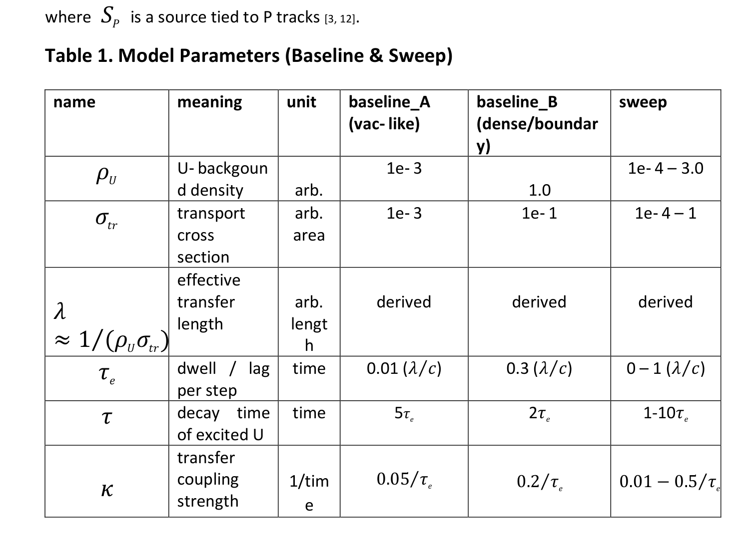
where 𝑆𝑃 is a source tied to P tracks [3, 12].

Table 1. Model Parameters (Baseline & Sweep)

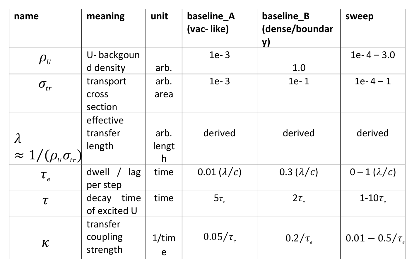
name meaning unit baseline_A (vac‑ like)

sweep

baseline_B (dense/boundar y)

𝜌𝑈 U‑ backgoun d density

1e‑ 3 1.0

1e‑ 4 – 3.0

arb.

1e‑ 3 1e‑ 1 1e‑ 4 – 1

𝜎𝑡𝑟 transport cross section

arb. area

𝜆 ≈1 (𝜌𝑈𝜎𝑡𝑟) ⁄

effective transfer length

derived

derived

derived

arb. lengt

h

time 0.01 (𝜆𝑐 ⁄ ) 0.3 (𝜆𝑐 ⁄ ) 0 – 1 (𝜆𝑐 ⁄ )

𝜏𝑒 dwell / lag per step

𝜏 decay time of excited U

time 5𝜏𝑒 2𝜏𝑒 1-10𝜏𝑒

𝜅

0.01 −0.5 𝜏𝑒 ⁄

transfer coupling strength

0.05 𝜏𝑒 ⁄

0.2 𝜏𝑒 ⁄

1/tim

e

𝑟𝑐

transfer radius

lengt

0.1 −1.0𝜆

0.5𝜆

0.8𝜆

h

𝑝(𝜃)

forward‑ peake d

scattering kernel (P→U)

broadened (near‑ Lambertia n)

—

HG g: 0.9 →0.0

𝑐 U‑ transfer critical speed

speed

1.0 (nondim) 1.0 fixed

𝜐𝑝 P speed (unobserved )

speed 1.5𝑐 1.2𝑐 ≥𝑐

𝜐𝑒𝑓𝑓 = 1 (1 𝑐 + ⁄ ⁄ 𝜏𝑒𝜆) ⁄

effective propagation speed

speed

computed

computed

computed

𝑛 = 1 + 𝑐𝜏𝑒𝜆 ⁄

effective refractive index

—

≈ 1.01

≈ 1.3

1.0 − 2.0

𝜏𝑐 sync time for interference

time 100𝜏𝑒 50𝜏𝑒 10 − 200𝜏𝑒

𝐿𝑐 =

coherence length

lengt

computed computed computed

h

𝜐𝑒𝑓𝑓𝜏𝑐

𝛥𝑡𝑖𝑛𝑡 detector integration window

time

50𝜏𝑒

50𝜏𝑒

10 − 200𝜏𝑒 observable

𝛥𝑇, 𝑉, 𝑛𝑒𝑓𝑓 —

measure

measure

record vs

s

sweep

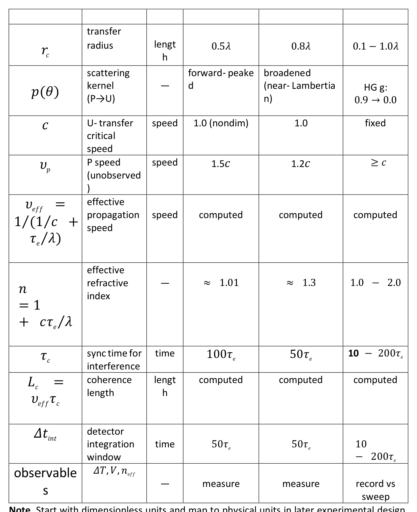
Note. Start with dimensionless units and map to physical units in later experimental design. Baseline_A is vacuum‑ like; Baseline_B represents strong boundary/scattering conditions [3,

12].

Table 2. Numerical Settings (Recommended)

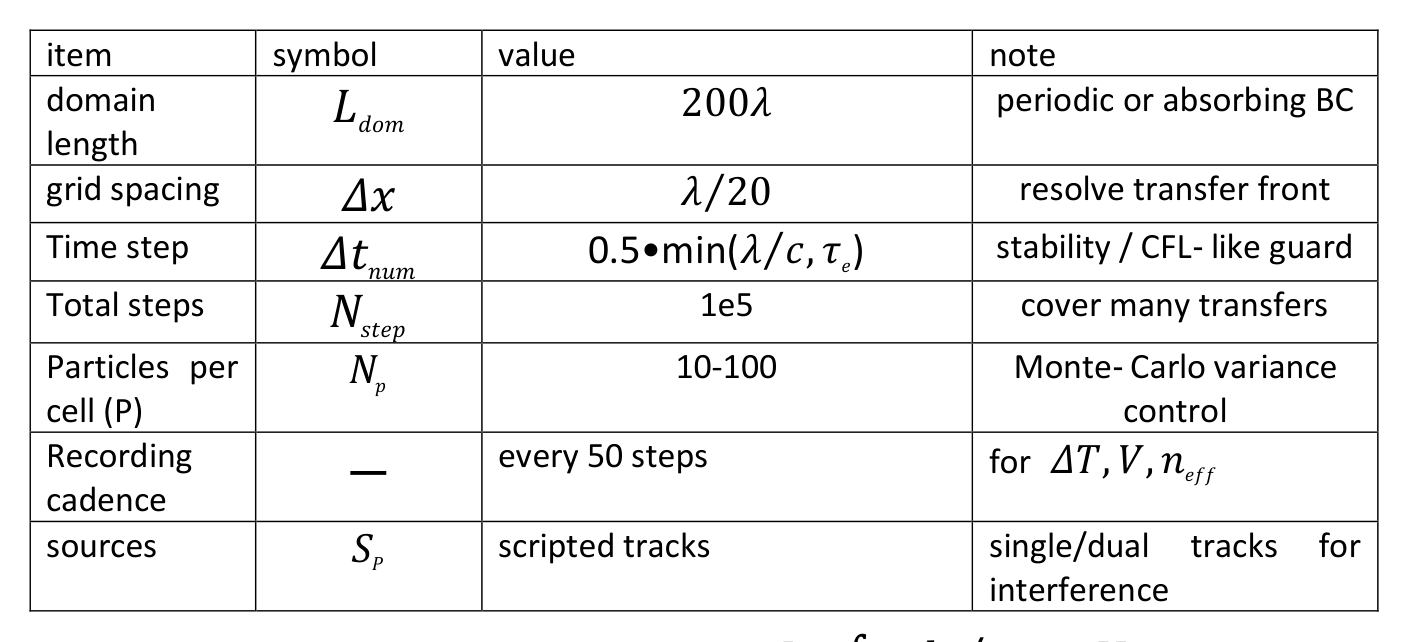
item symbol value note domain length 𝐿𝑑𝑜𝑚 200𝜆 periodic or absorbing BC

grid spacing 𝛥𝑥 𝜆20 ⁄ resolve transfer front

Time step 𝛥𝑡𝑛𝑢𝑚 0.5•min(𝜆𝑐, 𝜏𝑒 ⁄ ) stability / CFL‑ like guard

Total steps 𝑁𝑠𝑡𝑒𝑝 1e5 cover many transfers

𝑁𝑝 10-100 Monte‑ Carlo variance

Particles per cell (P)

control Recording cadence − every 50 steps for 𝛥𝑇, 𝑉, 𝑛𝑒𝑓𝑓

sources 𝑆𝑃 scripted tracks single/dual tracks for interference

Output metrics. 𝛥𝑇: time delay across length 𝐿 (∫ 𝑑𝑠𝜈𝑒𝑓𝑓 ⁄ ); 𝑉: fringe visibility (𝐼𝑚𝑎𝑥−𝐼𝑚𝑖𝑛) (𝐼𝑚𝑎𝑥+ 𝐼𝑚𝑖𝑛) ⁄ ; 𝑛𝑒𝑓𝑓 : path‑ averaged refractive index

(1 𝐿 ⁄ ) ∫ 𝑛(𝑠)𝑑𝑠.

8. Experimental Predictions and Discriminators

1. Pressure/density‑ dependent index. Control residual gas (affecting 𝜆, 𝜏𝑒) and measure 𝛥𝑇 ~ 𝐿𝛥(𝜏𝑒𝜆 ⁄ ) [2, 3, 12].

2. Boundary dynamics. Design interfaces (metasurfaces) to tailor 𝑝(𝜃) , inducing

non‑ integer refraction and polarization‑ dependent 𝑛 [3, 11].

3. Time‑ synchronization interferometry. Scan pulse delay and locate the threshold 𝜏𝑐 for fringe onset [2, 7].

4. UHV gas‑ injection step test. Micro‑ step 𝜆, 𝜏𝑒 by controlled injections and read out

femto–picosecond timing shifts via interferometry: 𝛥𝑛 ≈ 𝑐𝛥(𝜏𝑒𝜆 ⁄ ) [2 ,3, 4].

5. Kernel engineering at boundaries. Actively vary 𝑝(𝜃) and compare with ITFC predictions (cascade‑ transfer delays) [3, 11].

6. Annual/azimuthal modulation interferometry. Possible large-scale background modulation may be explored through annual or azimuthal interferometric variation, but such effects are not essential to the present local phenomenology of excitation transfer..

9. Mapping to Topological Terminology (Optional)

U‑ background corresponds to a near‑ zero phase‑ feedback exterior of a quasi‑ isolated system; contact transitions are phenomenologically analogous to entropy‑ direction inversions. This gives a dictionary between excitation-based and phase-based language without altering predictions..

9.1 Phase Symmetry in Nuclear Binding and Phase Relaxation (Beta Decay)

We interpret nuclear binding as a tendency to maintain phase symmetry (or equilibrium) within a bound system.

Let 𝛷𝑖 and 𝛷𝑗 denote the phases of nucleons i and j, and introduce a short-range envelope

𝑈(𝑅𝑖𝑗) ~ −𝐽0𝑒𝑥𝑝(−𝑅𝑖𝑗𝜆𝑁) ⁄ . A phenomenological binding energy can be written as:

𝐸𝑏𝑜𝑛𝑑 = −∑𝐽𝑖𝑗(𝑅𝑖𝑗)𝑐𝑜𝑠(𝜙𝑖 − 𝑠𝑖𝑗𝜙𝑗

<𝑖,𝑗>

− 𝜋𝑝𝑖𝑗) + ∑𝑈(𝑅𝑖𝑗)

<𝑖,𝑗>

where 𝑠𝑖𝑗 ∈ {±1} represents the coupling sign (in-phase or anti-phase), and

𝑝𝑖𝑗 ∈ {0,1} encodes a π-junction (e.g., neutron-mediated anti-phase coupling).

Energy minimization enforces local phase equilibrium, naturally producing

short-range strong attraction and saturation behavior [8, 9, 10].

In this framework, beta decay is interpreted as a phase relaxation (phase-slip) process

that occurs when accumulated phase imbalance exceeds a critical barrier.

Introducing an isospin angle α with an effective potential:

𝑈𝑖𝑠𝑜(𝛼) = −𝐽𝑝𝑛𝑐𝑜𝑠𝛼 + 𝐾

a phase-slip transition 𝛼 → 𝛼 ± 𝜋 occurs when the phase energy exceeds a

threshold 𝐸𝑏.

The released energy is partitioned as:

𝑄 = ∆𝐸𝑝ℎ𝑎𝑠𝑒 − 𝐸𝑏

= 𝑇𝑒 + 𝑇𝜈 + 𝐸𝑈−𝑐𝑎𝑠𝑐𝑎𝑑𝑒 ≥ 0

where 𝑇𝑒 and 𝑇𝜈 denote the kinetic energies of the emitted electron and (anti)neutrino,

and the remaining energy is carried by the U-cascade (flash chain) [8, 9, 10].

Charge conservation is ensured via the label-charge continuity relation

(Appendix D.5′):

𝜕𝑡𝜌𝑞 + 𝛻 ∙ 𝐽𝑞 = 𝑆𝑠𝑙𝑖𝑝

which reduces to standard conservation (𝑆𝑠𝑙𝑖𝑝 → 0) in the rapid recombination limit.

Thus, beta decay is interpreted as a dynamical process restoring phase equilibrium

within the bound system.

10. Limitations and Open Problems

• Establish a precise effective field theory mapping to Maxwell/QED [1, 5, 6, 9].

• Quantitatively confront high‑ precision null experiments [4].

• Integrate a nonlinear detector model for biological perception.

11. Conclusion

ITFC redefines light as a cascade of localized 𝑈∗ excitations and their emitted flashes, and

interprets the light constant as a U‑ transfer critical speed. Thus, while a driver P may satisfy 𝜐𝑃 ≥𝑐, information transfer remains bounded by 𝜐𝑒𝑓𝑓 ≤𝑐. Medium sensitivity is

quantified by 𝑛 = 1 + 𝑐𝜏𝑒𝜆 ⁄ . The frame unifies rectilinearity, reflection/refraction, scattering/turbidity, and diffraction/interference through the single spatial field 𝜏𝑒𝜆 ⁄ . We propose UHV step tests and boundary‑ kernel engineering as near‑ term discriminators.

In addition to its optical interpretation, the ITFC framework may be read as a phenomenological background-excitation model. In this view, observable propagation is determined by the transfer of localized excitations through unobservable background degrees of freedom. Possible large-scale background modulation may be explored in future work, but it is not essential to the present formulation, which is primarily concerned with the local phenomenology of light propagation.

Future work. (1) Construct a microscopic background-excitation model and an EFT correspondence; (2) infer the effective parameters from metasurface/nanointerferometry datasets; (3) perform precision comparisons of the main observables; (4) explore possible large-scale background-modulation effects through refractive-index mapping.

---

Appendix A. Covariant Parameter‑Scaling Hypothesis (Sketch)

In local inertial frames, let 𝜆 ∝ 𝑓(𝛷) and 𝜏𝑒 ∝ 𝑓(𝛷) scale homogeneously with a local scalar 𝛷, keeping . Then 𝜐𝑒𝑓𝑓

−1 = 𝑐

−1 + 𝑐𝑜𝑛𝑠𝑡 is locally invariant and first‑ order anisotropy cancels.

Appendix B. Notation

𝜌𝑈: density of background degrees of freedom; 𝜎: (transport) cross section; ℓ: transport mean free path; 𝜆: effective transfer length; 𝜏, 𝜏𝑒: decay/dwell constants; 𝜅: transfer coupling; 𝑟𝑐: transfer radius; 𝑐: U‑ transfer critical speed; 𝑛: effective refractive index; 𝑢

∗: excited U concentration; 𝜐𝑃: P speed; 𝜐𝑒𝑓𝑓: effective cascade speed.

Appendix C. Diagrams (v1)

Display note. If Mermaid is unavailable, use the ASCII alternates. Variables appear in plain text (tau_e, lambda, r_c).

[Fig. 1] U‑ cascade propagation (P track and excitations)

flowchart LR

P0((P)) --> U1((U*))

U1 --> U2((U*))

U2 --> U3((U*))

P0 -. dotted path .-> P1((P))

P1 --> U4((U*))

U4 --> U5((U*))

classDef glow fill:#fffbd6,stroke:#555;

class U1,U2,U3,U4,U5 glow;

ASCII alt:

P path: . . . . . . . . .

o* -> o* -> o* (U* : excited U; flash)

\

-> o* -> o*

r_c : local transfer radius

lambda : effective transfer length between successive U*

[Fig. 2] Trajectory change at a boundary (refraction/reflection)

flowchart LR

subgraph A[region A: n_A = 1 + c*tau_eA/lambda_A]

IA[/incident ray θ_A/]

end

subgraph B[region B: n_B = 1 + c*tau_eB/lambda_B]

RB[/refracted ray θ_B/]

end

IA -->|boundary| RB

ASCII alt:

region A (n_A) | region B (n_B)

\

\ θ_A | / θ_B

\____boundary|_/________

Snell: n_A * sin(θ_A) = n_B * sin(θ_B)

with n = 1 + c * tau_e / lambda

[Fig. 3] Time‑ synchronization interference (coherence length L_c)

P-chain #1: |* * * * *|

P-chain #2: |* * * * *|

<---- Δt ---->

Detector window Δt_int: [===========]

Sync time τ_c: threshold for fringe formation

L_c = v_eff * τ_c = c * τ_c / (1 + c * tau_e / lambda)

Appendix D. Effective Action (Lagrangian) — Sketch

This appendix presents a refined effective action sketch for ITFC while preserving the phenomenological parameters 𝜆, 𝜏𝑒, 𝜏𝑠𝑤𝑎𝑝, 𝜅. The purpose is twofold: (i) encode memory effects and finite transfer range directly in the action, and (ii) to recover, in the long‑ wavelength and low‑ frequency limit, the ITFC propagation law

𝑡𝑠𝑡𝑒𝑝 = 𝜆

𝑐 + 𝜏𝑒𝑓𝑓,

𝜐𝑒𝑓𝑓 = 1 𝑐−1 + 𝜏𝑒𝑓𝑓𝜆 ⁄ ,

𝑛 = 1 + 𝑐𝜏𝑒𝑓𝑓

𝜆

Where

𝜏𝑒𝑓𝑓 = {𝜏𝑒 , 𝑑𝑖𝑙𝑢𝑡𝑒 𝑏𝑎𝑐𝑘𝑔𝑟𝑜𝑢𝑛𝑑,

𝜏𝑠𝑤𝑎𝑝, 𝑑𝑒𝑛𝑠𝑒 𝑠𝑤𝑎𝑝−𝑑𝑜𝑚𝑖𝑛𝑎𝑡𝑒𝑑 𝑏𝑎𝑐𝑘𝑔𝑟𝑜𝑢𝑛𝑑.

The effective action introduced in Appendix D is not presented as a complete microscopic quantum theory, but as a coarse-grained phenomenological model compatible with a quantum-interpreted background picture.

D.1 Fields and External Source

Let 𝜓(𝑥) ≡ 𝜓(t, r) denote an effective scalar field representing the intensity/state of U- transfer, I.e. the observable carrier of the U-cascade. The P-track enters only through an external source

𝐽𝑝(𝑥) = 𝑔∫𝑑𝜏 𝛿(4)(𝑥 − 𝑋(𝜏)),

where 𝑋(𝜏) is the worldline of the P-particle. Thus, P itself is not directly observable; only

the induced field 𝜓 is.

D.2 Effective Action (Sketch)

The refined effective action is written as

𝑆𝑒𝑓𝑓 = ∫𝑑4𝑥 [1

2 (𝜕𝑡𝜓)2 − 𝑐2

2

2 ∣𝛻𝜓∣

− 𝑉(𝜓) + 𝐽𝑃𝜓]

+ 1

2 ∫𝑑4𝑥𝑑4 𝑥′𝜓(𝑥)𝐾(𝑥−𝑥′)𝜓(𝑥′).

Here 𝛫(𝑥 − 𝑥′) is a causal nonlocal kernel satisfying

𝐾(𝑡 − 𝑡′ < 0, 𝑟 − 𝑟′) = 0,

so that temporal ordering and observable causality are preserved.

A separable illustrative form is

𝐾(𝑥 − 𝑥′) = 𝐾𝑡(𝑡 − 𝑡′) 𝐾𝑟(𝑟 − 𝑟′),

with

𝐾𝑡(∆𝑡) = 𝛼

𝑒𝑥𝑝(−∆𝑡

) 𝛩(∆𝑡),

𝜏𝑒𝑓𝑓

𝜏𝑒𝑓𝑓

𝑒𝑥𝑝(−∣∆𝑟∣𝜆) ⁄

𝑐

𝐾𝑟(∆𝑟) = −𝛽

𝜆

𝑁𝜆 ,

where 𝑁𝜆 is a normalization factor and 𝛼, 𝛽 are matching coefficients.

If a cosmic reversible rotation field 𝛺 = 𝛺(𝑅) is included, the kernel may be parameterized as

𝐾(𝑥 − 𝑥′; 𝛺)

= 𝐾𝑡(𝑡 − 𝑡′; 𝛺)𝐾𝑟(𝑟 − 𝑟′; 𝛺),

with Fourier transform

𝐾̃(𝜔, 𝑘; 𝛺)

≃ 𝐴(𝛺)(𝑖𝜔) + 𝐵(𝛺)𝑘2 + ⋅⋅⋅ .

The matching conditions are then imposed as

𝜕𝐾̃

𝜕𝐾̃

1

𝑐

(

𝜕(𝑖𝜔))

=

𝜏𝑠𝑤𝑎𝑝(𝛺), (

𝜕𝑘2)

𝜔=0,𝑘=0 = −

𝜆(𝛺)

𝜔=0,𝑘=0

These ensure the long-wavelength relations

𝑐𝜏𝑠𝑤𝑎𝑝(𝛺)

1

𝜐𝑒𝑓𝑓(𝛺) =

𝑐−1 + 𝜏𝑠𝑤𝑎𝑝(𝛺) 𝜆(𝛺) ⁄ , 𝑛(𝛺) = 1 +

𝜆(𝛺)

D.3 Equations of Motion and Dispersion (Linearized)

Near a local steady state, take

𝑉(𝜓) ⋍ 𝑚2

2 𝜓2.

Then the Euler–Lagrange equation becomes

𝜕𝑡

2𝜓 − 𝑐2𝛻2𝜓 + 𝑚2𝜓

+ ∫𝑑4𝑥′ 𝐾(𝑥 − 𝑥′)𝜓(𝑥′)

= −𝐽𝑃(𝑥).

For a plane-wave ansatz

𝜓(𝑥) ~ 𝑒𝑖(𝑘⋅𝑟 − 𝜔𝑡),

one obtains the dispersion relation

−𝜔2 + 𝑐2𝑘2 + 𝑚2 + 𝐾̃(𝜔, 𝑘) = 0.

In the long‑ wavelength/low‑ frequency regime,

𝐾̃(𝜔, 𝑘) ≈ 𝐴(𝑖𝜔) + 𝐵𝑘2 + ⋅⋅⋅ ,

And the coefficients 𝐴 and 𝐵 are fixed by the ITFC matching rules below.

D.4 Long‑ Wavelength Matching (Design Rules)

The refined design rules are:

(𝑀1) 𝑡𝑠𝑡𝑒𝑝 = 𝜆

𝑐 + 𝜏𝑒𝑓𝑓 ⇒ 𝜐𝑓𝑟𝑜𝑛𝑡

= 1 𝑐−1 + 𝜏𝑒𝑓𝑓𝜆 ⁄ ≡ 𝜐𝑒𝑓𝑓 ,

(𝑀2) 𝑛 = 𝑐 𝜐𝑒𝑓𝑓

= 1 + 𝑐 𝜏𝑒𝑓𝑓

𝜆 ,

(𝐶1) ( 𝜕𝐾̃

= 1

,

𝜕(𝑖𝜔))

𝜏𝑒𝑓𝑓

0

(𝐶2) (𝜕𝐾̃

= − 𝑐

𝜆 .

𝜕𝑘2)

0

Choosing 𝛼, 𝛽, and 𝑁𝜆 so that (𝐶1) −(𝐶2) hold ensures that the front velocity of the causal U-cascade response reproduces the ITFC law.

> Remark. In a generic nonlocal medium, phase velocity and group velocity need not coincide with the signal front velocity. In ITFC, the physically relevant quantity is the propagation of

the U-cascade front.

D.5 Minimal Potential and Stability

A stable minimal potential may be chosen as

𝑉(𝜓) = 𝑚2

2 𝜓2 + 𝜆4

4! 𝜓4 + ⋅⋅⋅, 𝑚2

≥ 0, 𝜆4 ≥ 0.

If one prefers a phase interpretation, a periodic form such as

𝑉(𝜙) = 𝛬𝜙(1 − 𝑐𝑜𝑠𝜙)

may be used instead.

D.5’ Label-Charge Continuity (Noether Sketch)

Assume a global 𝑈(1)-like symmetry associated with a label charge 𝑞. Then the effective current obeys

𝜕𝑡𝜌𝑞 + 𝛻 ⋅ 𝐽𝑞 = 0.

D.6 Summary

The refined effective action preserves:

(1) 𝑐𝑎𝑠𝑢𝑎𝑙𝑖𝑡𝑦, (2) 𝑓𝑖𝑛𝑖𝑡𝑒 𝑚𝑒𝑚𝑜𝑟𝑦 / 𝑟𝑎𝑛𝑔𝑒 (𝜏𝑒𝑓𝑓, 𝜆), (3) 𝑖𝑛𝑣𝑎𝑟𝑖𝑎𝑛𝑡 𝑐.

in the long-wave-length limit. In laboratory vacuum without pair production, any effective-

mass construct may be set to zero, and the pair (𝜆, 𝜏𝑒) alone suffices. A full microscopic

derivation and EFT correspondence remain future work.

References

[1] Maxwell, J. C., *A Treatise on Electricity and Magnetism*, Vols. I–II, Clarendon Press, Oxford (1873).

[2] Born, M. and Wolf, E., *Principles of Optics: Electromagnetic Theory of Propagation, Interference and Diffraction of Light*, 7th expanded ed., Cambridge University Press (1999).

[3] Landau, L. D., Lifshitz, E. M., and Pitaevskii, L. P., *Electrodynamics of Continuous Media*, 2nd ed., Butterworth-Heinemann / Elsevier, Vol. 8 of Course of Theoretical Physics (1984).

[4] Michelson, A. A. and Morley, E. W., “On the Relative Motion of the Earth and the Luminiferous Ether,” *American Journal of Science* **34**(203), 333–345 (1887).

[5] Feynman, R. P., *QED: The Strange Theory of Light and Matter*, Princeton University Press (1985).

[6] Jackson, J. D., *Classical Electrodynamics*, 3rd ed., Wiley (1998).

[7] Hecht, E., *Optics*, 5th ed., Pearson (2016).

[8] Sakurai, J. J. and Napolitano, J., *Modern Quantum Mechanics*, 2nd ed., Cambridge University Press (2017).

[9] Peskin, M. E. and Schroeder, D. V., *An Introduction to Quantum Field Theory*, CRC Press / Westview Press (1995).

[10] Weinberg, S., *The Quantum Theory of Fields*, Vol. I, Cambridge University Press (1995).

[11] Joannopoulos, J. D., Johnson, S. G., Winn, J. N., and Meade, R. D., *Photonic Crystals: Molding the Flow of Light*, 2nd ed., Princeton University Press (2008).

[12] Ishimaru, A., *Wave Propagation and Scattering in Random Media*, Vols. I–II, Academic Press (1978).